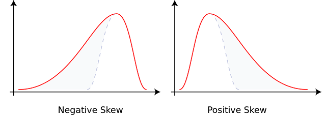
Methods of determining Skewness and the
coefficient of Skewness.
If a frequency curve of a given frequency
distribution is drawn, then it can be known whether the skewness is
positive or negative. But the numerical measure of skewness can not be known.
Also, it is necessary to find numerical measures of skewness for comparison of
two or more frequency distributions. For determining skewness and the
coefficient of skewness following two methods are used.
(I) Karl Pearson’s Method
(II) Bowley’s Method
(1) Karl Pearson’s Method:
Base: In a skewed frequency distribution, the
values of the mean, median, and mode are not equal i.e. X̅ not equal to M not equal to Z. Also, the median always lies between
the mean and mode. Karl Pearson’s method is based on this test of skewness.
Formulae: Skewness is the difference between the mean
and mode.
i.e. skewness (sk) = X̅ - Z
The coefficient of skewness is obtained by
dividing the above difference by standard deviation (S).
i.e. coefficient of Skewness (j) = X̅
- Z / S
When the frequency distribution is not unimodal
or otherwise the mode is ill-defined, then mode can be obtained by the formula Z
= -3M – 2X̅
Hence, when a mode is ill-defined then the following
formulae are used.
Skewness (sk) = 3 (X̅ - M)
Coefficient of Skewness (j) = 3 (X̅ - M)
/ S
Note:
(i) The value of the coefficient of skewness given by
formula 3 ( X̅ - M) / S always lies between between
-1.73 and +1.73 for any uni-modal skewed frequency distribution.
This
has been proved by statistician N.L. Johnson in the year
1951. But generally, in practice, the value of j based on a sample lies
between -1 and +1 for skewed frequency distribution.
(ii)
The value of the coefficient of skewness given by formula j = 3 ( X̅ - M) / S always lies between
-3 and +3.
(iii) The mode is said to be ill-defined in the
following situation:
(a) if the frequency distribution has classes
of unequal length.
(b) if the frequency distribution is a mixed
type (partly discrete and partly continuous).
(c) If the frequency distribution has been more
than one mode. In this situation, the following formulae are used.
sk = 3 (X̅ - M) and j = 3 (X̅ - M) / S
(2) Bowley’s Method :
Base: In a skewed frequency distribution, both the
quartile Q1 and Q3 are not equi-distant from the median.
i.e. Q3 – M not equal to M – Q1. Bowley’s method is based on this
test of skewness.
Formulae: The difference between the distance Q3
– M and M – Q1 is taken as the
absolute measure of skewness (sk).
i.e. Skewness (sk) = (Q3 – M) – (M – Q1)
= Q3 – M – M + Q1
Skewness
(sk) = Q3 + Q1 – 2M
The coefficient of
skewness is obtained by dividing the above difference by the sum of the
distance Q3
– M and M – Q1.
coefficient of
skewness (j) = Q3
+ Q1 – 2M / Q3 - Q1
Note: the value of the coefficient
of skewness (j) given by Bowley’s method always lies between -1 and +1.
Comparison of Karl
Pearson's Method and Bowley's Method.
1. As Karl Pearson's method and
Bowley's method are based on different assumptions, the values of the
coefficient of skewness obtained by the two methods may not be equal.
2. The calculations are simple and easy in
Bowley's method, whereas the calculations are not simple in taking more time in
Karl Pearson's method.
3. The co-efficient of skewness obtained
by Karl Pearson's method is more reliable than Bowley's method. Karl
Pearson's formula off is based on mean X and standard deviation (S) which are the
best measures of average and dispersion.
4. Karl Pearson's method cannot be used
for open-end frequency distribution. When open-end frequency distribution is
given then Bowley's method is to be used.
Points to be
remembered while solving examples
(1) If it is not
stated by which method co-efficient of skewness is to be calculated in the
example, then use Karl Pearson's method.
(2) If the frequency
distribution is open-end frequency distribution, then use Bowley's method for
calculating the coefficient of skewness.
(3) In a given
frequency distribution, the observations or the classes are to be arranged in
ascending order if they are not in ascending order.
(4) If the classes of
a given frequency distribution are exclusive, then find boundary points for the
corresponding classes for calculating median, mode, or quartiles.
(5) If the cumulative
frequency distribution of 'less than type' or 'more than type' is given, then
convert it into an original frequency distribution.
(6) If instead of
classes, the mid-values are given then first find boundary points for
each mid-value by the
following formulae.
Lower boundary point
= Mid-value - (Class interval / 2)
Upper boundary point
= Mid-value + (Class interval / 2)
(7) If mode is
ill-defined, then for Karl Pearson's method use the following formulae.
sk = 3 (X̅
- M) and j = 3 (X̅ - M) / S
(8) If a given
frequency distribution is of unequal class interval or of mixed type i.e.
partly discrete and partly continuous, then for calculation of mean and
standard1 deviation by short cut method class interval (C) should not be taken.
(9) The value of the
coefficient of skewness may be positive, negative, or zero.


